
Deep-Learning-Based Object Filtering According to Altitude for Improvement of Obstacle Recognition during Autonomous Flight


Department of Computer Science, Hanyang University, Seoul 04763, Korea
*
Author to whom correspondence should be addressed.
Remote Sens. 2022, 14(6), 1378; https://doi.org/10.3390/rs14061378
Submission received: 26 January 2022
/
Revised: 3 March 2022
/
Accepted: 7 March 2022
/
Published: 12 March 2022
(This article belongs to the Special Issue AI Interpretation of Satellite, Aerial, Ground, and Underwater Image and Video Sequences)
Abstract
:The autonomous flight of an unmanned aerial vehicle refers to creating a new flight route after self-recognition and judgment when an unexpected situation occurs during the flight. The unmanned aerial vehicle can fly at a high speed of more than 60 km/h, so obstacle recognition and avoidance must be implemented in real-time. In this paper, we propose to recognize objects quickly and accurately by effectively using the H/W resources of small computers mounted on industrial unmanned air vehicles. Since the number of pixels in the image decreases after the resizing process, filtering and object resizing were performed according to the altitude, so that quick detection and avoidance could be performed. To this end, objects up to 60 m in height were classified by subdividing them at 20 m intervals, and objects unnecessary for object detection were filtered with deep learning methods. In the 40 m to 60 m sections, the average speed of recognition was increased by 38%, without compromising the accuracy of object detection.
1. Introduction
The autonomous flight of an Unmanned Aerial Vehicle (UAV) refers to creating a new flight route after self-recognition and judgment when an unexpected situation occurs during the flight. In the case of the UAV, the recognition and judgment of the UAV are used to measure the distance or avoid obstacles through object recognition by receiving data from various sensors such as a single camera [1,2,3], a depth camera [4,5,6], LiDAR [7,8], an ultrasonic sensor [9,10], or radar [11]. Furthermore, rather than employing a single sensor, complex sensors are increasingly being employed to compensate for the shortcomings of each sensor. Vision-based, ultrasonic, and infrared sensors are some of these, and if they fail due to the temperature or illumination circumstances, they might result in collisions. As a result, highly reliable industrial drones typically utilize a complicated sensor strategy. As computer vision and machine learning techniques progress, vision-sensor-based autonomous flight is becoming increasingly widespread. The drone sends data from sensors such as the three-axis gyroscope, three-axis accelerometer, magnetometer, GNSS, or barometer to the Flight Control Computer (FCC), which calculates the drone’s posture and keeps it stable in the air [12]. Accordingly, a separate Companion Computer (CC) is mounted to perform computing for image processing and autonomous flight. Unless it is a large Predator-class fixed-wing drone, the size and weight of the CCs are very important because most drones have little space to mount electronic parts. The CC used is mainly from the Raspberry Pi family and NVIDIA’s Jetson series for hobbies and development purposes. In particular, the Jetson model group includes a basic GPU and is small in size and light in weight, so even when mounted on a drone, the flight time is not significantly reduced, making it suitable as a CC for autonomous flight, object detection, and object tracking. In addition, autonomous drones recently released for hobbies or personal use are about USD 1000, and the price of realistic CCs must be considered, so development using Nano products among the Jetson models is actively underway. The Nano is small and has an excellent performance in graphic operation processing. However, detecting hundreds of objects among high-resolution images transmitted in real-time will inevitably lead to frame degradation. Drones can detect obstacles only when a minimum frame rate is guaranteed in proportion to the flight speed.
Drones with rotary blades often fly at speeds of 10–30 m/s; however, if the frame rate drops due to a long duration, they will fly in a blackout situation and collide with obstacles. As a result, the speed with which drones detect objects in real-time is critical. As shown in Figure 1, the higher the Frames Per Second (FPS), the more images are processed and displayed. It is necessary to go through a preprocessing step when processing an image so that the CC can quickly perform an object recognition process with the images.
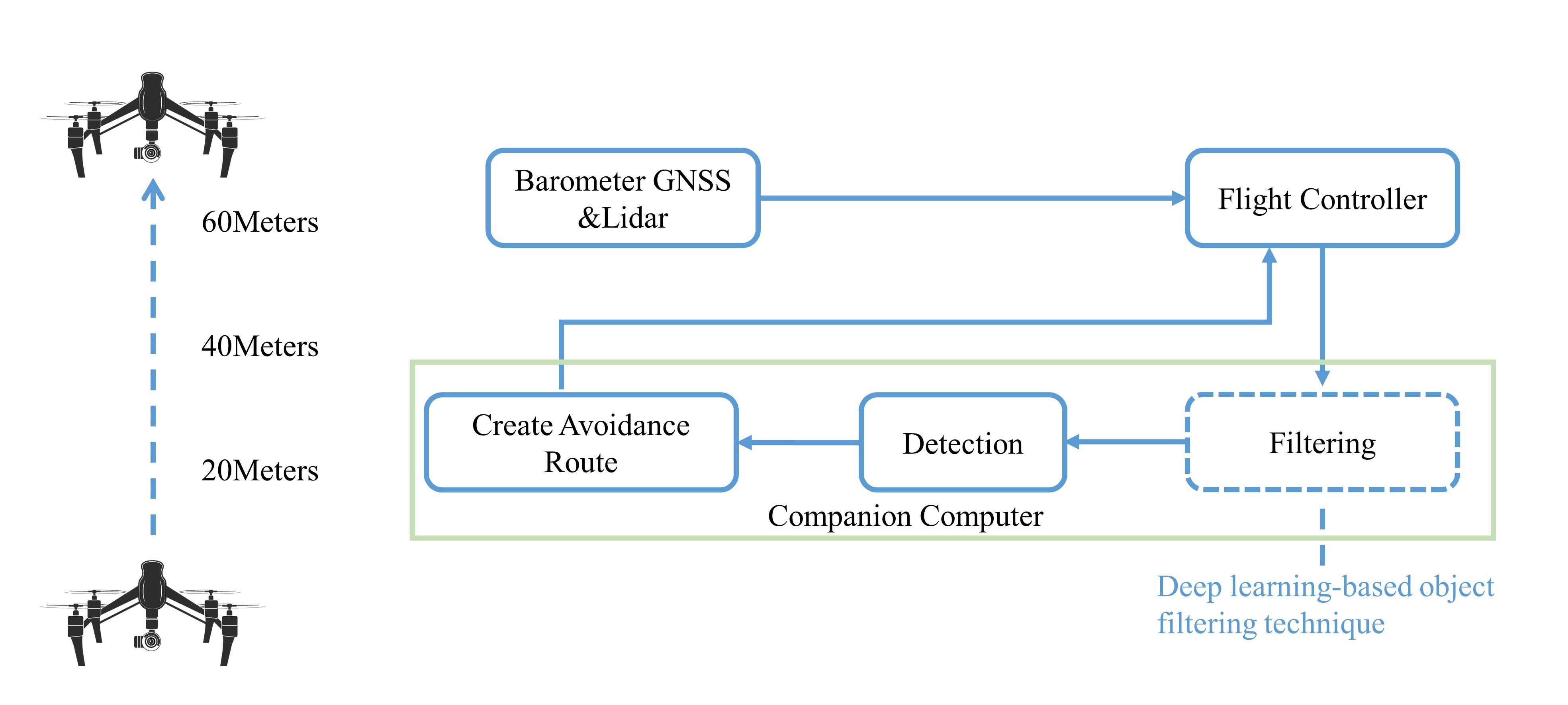
In the case of Figure 2, the performance of various deep learning models for inference is shown. The time taken to detect one frame is called the inference time. The SSD-ResNet [13], SSD-Mobilenet [14], and YOLOv3 [15] models have shown good performance and a high frame rate in object detection tasks. The R-CNN series takes a long time because it separates and analyzes multiple photos using the CNN model; however, the YOLO family is quick because it just searches once. YOLOv3 is a model with and especially low mAP. Some researchers improved the performance of YOLOv5 [16] by upgrading the backbone architecture. YOLOv5’s backbone uses cross-stage partial networks [17] to extract feature maps from a given input image, which was developed as a new backbone that can improve the CNN’s performance.
In this paper, we tested several object detection models with data augmentation based on the VisDrone2019 dataset and AU-AIR dataset. The object detection models we tested were RetinaNet (Resnet50 backbone), the YOLO family, SSD, and others, while the augmented techniques we investigated included bilateral blurring, shifting to the HSV color space, cropping, dropout, elastic deformation, flipping, Gaussian blurring, and inverting. For the experiment results, the average inference time before filtering was 0.105 s, and the time after filtering was 0.066 s, which showed a performance improvement of about 59%.
2. Related Work
Studies using images from cameras during the autonomous flight of drones are being actively conducted. Traditional techniques include Simultaneous Localization And Mapping (SLAM) [18], which uses the difference in the position of the object in the image to obtain and coordinate depth information from two images, such as from stereo-cameras, that capture objects at different locations. Recently, a method of estimating depth and avoiding obstacles by using deep learning and installing monocular cameras was also studied [19]. This method can recognize objects even in spaces with a low texture. Existing ultrasonic sensors [20], LiDAR [7], IR sensors [21], and the above-mentioned stereo methods can resolve obstacles with high memory occupancy due to the data processing. Furthermore, small drones may overcome the limitations of the space that can be mounted. This technique first estimates the depth of the indoor environment based on the composite neural network and avoids obstacles based on this, and data augmentation techniques are used to preprocess the training data to improve the performance of the composite neural network. Data augmentation is a preprocessing technique that can prevent over-fitting and improve performance by augmenting the number of data through multiple conversions of the original to increase the amount of data. Among the data augmentation techniques, an image with a short average distance, various depths, and sufficient textures can be used to increase the performance by expanding the image and converting the colors for each RGB channel. As a result, the average distance of the image is between 2.5 m and 5 m; however, the environment is indoors, and the average distance is very short; therefore, it cannot be used for outdoors when flying at a high speed.
To improve object recognition performance in images, we can use training data enhancement. For the dataset, data are augmented and used as the training data by applying rotation, flipping, channel shifting, compression, blurring, and aspect size adjustment. In the preprocessing stage of the training data, the first step is to blur, dither, and add noise to the image with pixel-level transforms to improve performance and compensate for the training data, usually using motion blurring, Gaussian blurring, luminance dithering, ISO noise, and state dithering. For drones in flight, the data are changed by external factors such as the speed, weather, illuminance, camera distortion, and flight time. Therefore, even with data augmentation, the performance can be improved through conversion tasks similar to the flight environments. In addition to the data enhancement techniques, the transfer learning technique can be applied according to the characteristics of the training data. Transfer learning learns additional data by selecting a transfer learning method according to the characteristics of the training data and fine-tuning the weight of the model.
In this case [22], due to the lack of a drone dataset, ensemble transfer learning was used. As a result, multi-scale objects could be detected in the drone images. In the case of the VisDrone dataset, the best result was obtained on unmanned aerial vehicle datasets of custom models such as the DPNet-ensemble [23] and RRnet [24]. However, this approach does not utilize the concept of direct transfer learning in a baseline model independent of the target data and requires training on the target dataset, which is more time consuming and less efficient. Using these models with high accuracy, the ensemble learning technique changes the parameters and weighting, resulting in a 6.63% increase in the AU-AIR-dataset-based mAP compared to the previous deep learning model for the COCO dataset. In conclusion, the ensemble learning technique and augmentation technique for drone-based image datasets showed the possibility of performance improvement, and this was a worthwhile study based on the drone’s limited computing resources.
3. Methods
3.1. Requirements for Vision-Based Autonomous Flight
Vision-based Autonomous Flight (VAF) is a flight method that generally accepts images from optical cameras and processes them to avoid obstacles and autonomously fly. High-quality VAF is affected by the camera performance, image processing techniques, and computer specifications. The size of the drones increases, for example, as the distance between the shafts of the motor increases depending on the type of mission and payload, such as 0.3 m, 1 m, 2 m, and 5 m, and there are bound to be restrictions. Furthermore, trade-offs were made based on the size and performance. In this paper, we used object filtering techniques by altitude to improve the speed of obstacle recognition during the autonomous flight of industrial small drones.
The three main requirements for VAF drones can be described as follows: First, it should be a real-time detection. A fast model should be utilized to swiftly avoid barriers after they have been detected. Second, sensor fusion is needed to increase the accuracy of detection. VAF may be less accurate depending on the environment, for example the amount of sunlight, weather, or flight time, so it is necessary to increase the safety by adding sensors to compensate for this. Third, there is a need for a CC to process the autonomous flight of the drones. The drone was equipped with an FCC for flight control, which was only responsible for maintaining the drone’s posture. Therefore, a separate CC for object recognition was installed. However, above all, image processing must be performed, so the GPU-based performance must be supported to play the role as the CC.
3.2. Vision-Based Autonomous Flight Situations and Filtering Techniques
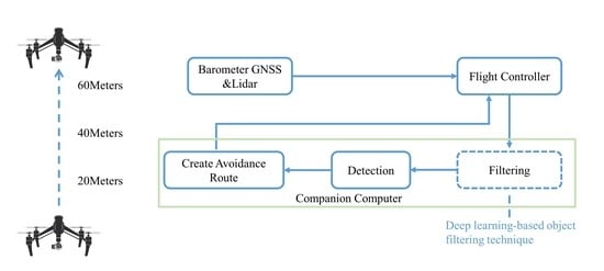
For the design and implementation of VAF, three situations were considered. First, drones flew vertically and horizontally from take-off to landing. In this situation, when flying vertically, the variety of objects depends on the flight height of the drone. In other words, the objects differed according to the height in the order of people, vehicles, traffic lights, streetlights, trees, bridges, and buildings from the ground. Second, as it rises, the variety of objects shrinks, and only large objects remain. The input image should be based on the front-view image, rather than the tilt-up or tilt-down image, which is the same as the composite sensor. Third, after it rises, large objects will be well detected because the shape is maintained even after resizing. If the size of objects in an image is small, the detection speed will be faster in the deep learning model because the number of pixels is small, so filtering and resizing objects by altitude can improve the detection speed while maintaining the accuracy. Furthermore, drones receive data from the gyroscope, accelerometer, magnetometer, GNSS, and barometer in real-time for posture control and deliver them to the FCC. In this situation, the altitude data are delivered from the GNSS and barometer, and LiDAR for the ranger finder function was used. In general, only the barometer and GNSS are used to have an error value of about 1 m, but when using a LiDAR, it is possible to measure the altitude with centimeter-level accuracy. Figure 3 shows the process of creating an avoidance route for VAF. Before performing the detection and recovery processes, a preprocessing was performed to reduce the processing time of the CC. For the filtering process, when the drone rises to an altitude of 20 m, the detected objects are classified. When the drone is between 20 m and 40 m high, smaller objects such as people and vehicles are filtered out. When the drone’s height is between 40 m and 60 m, it filter out other objects, and the photos to be input into the model are scaled.
3.3. Object Detection Using the Deep Learning Model
Deep learning models for object detection tasks can be classified into one-stage or two-stage models. A quick model for object detection that has one stage is necessary to avoid real-time drone collisions. From this perspective, we compared the models of the SSD family and the YOLO family. The workstation configuration for the experiment is given in Table 1.
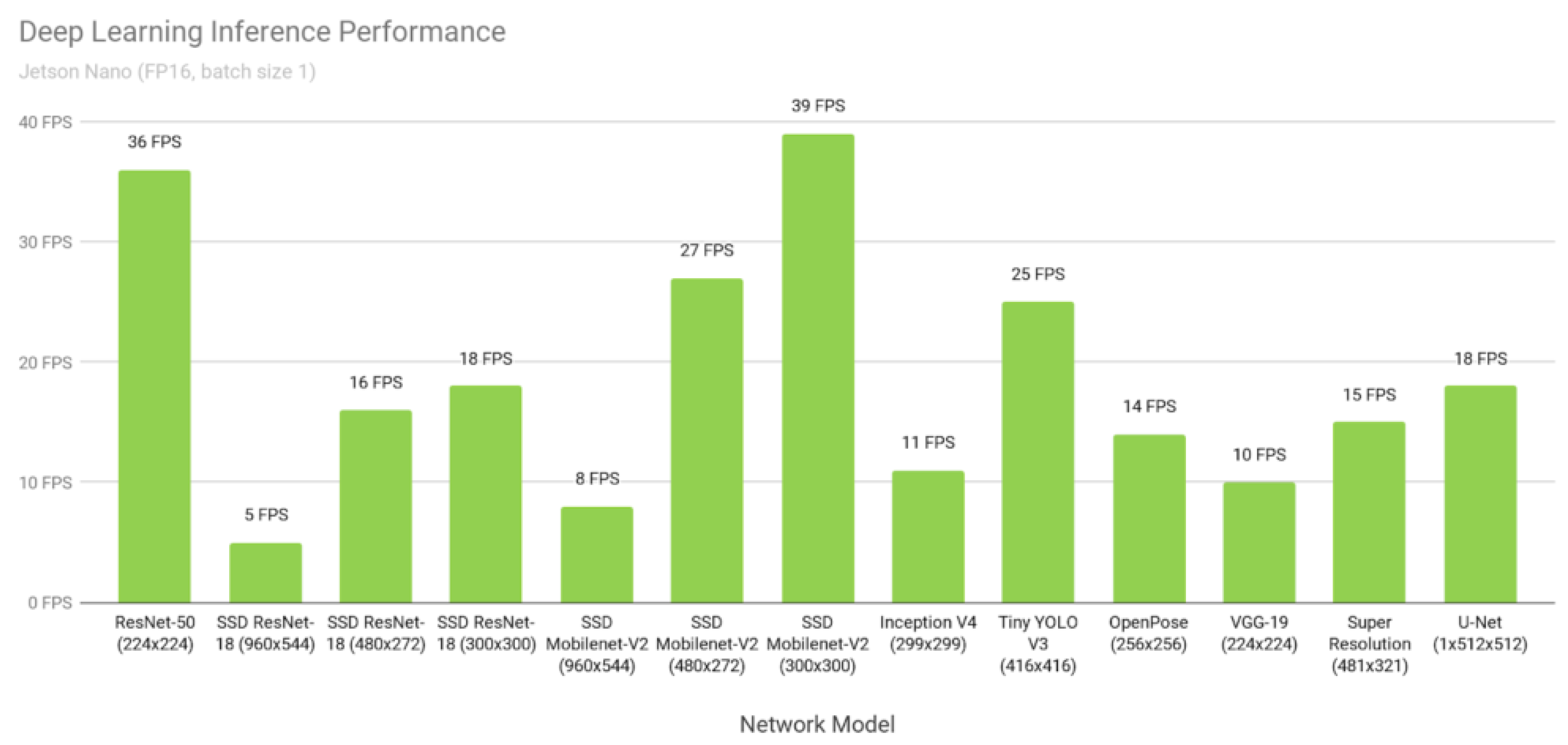
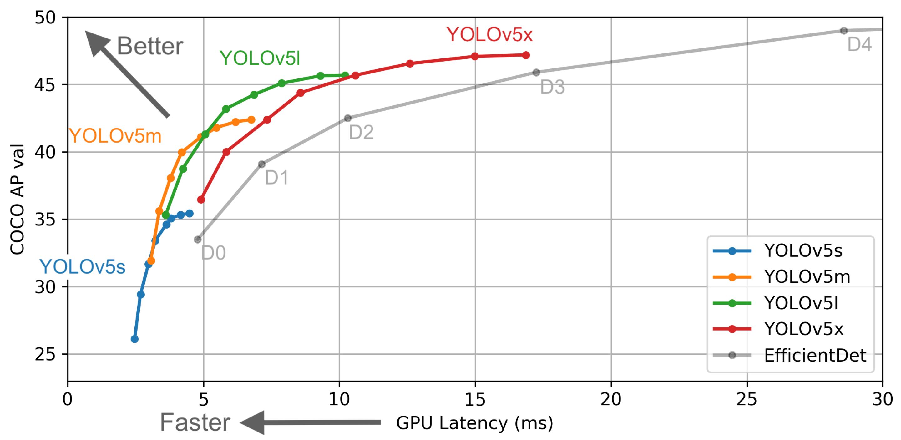
Table 2 shows the SSD family usually used at low FPS; this causes a long detection time, and the reason is that it divides several images and analyzes the images using the CNN model. On the contrary, the YOLO family runs fast because it searches only once. However, YOLOv3-tiny is a model with high FPS. Recently, the latest version of the YOLO family was published: YOLOv5. Figure 4 shows the performance of the mAP and FPS is improved due to some modifications to the model architecture. YOLOv5 is divided into four types: small (s), which has 12.7 million parameters, medium (m), which has 35.9 million parameters, large (l), which has 77.2 million parameters, and extra-large (x), which has 141.8 million parameters; these four types have the same backbone structure. This is directly related to the performance of the speed and accuracy, but there is a problem with the model slowing down as more resources are used. In this paper, we used the YOLOv5 small model, and for this, a real-time and light system were required, so we implemented our object detection using the YOLOv5 small model to ensure fast FPS.
3.4. Data Purification and Training the Model
The training dataset for object recognition was constructed based on the front fixed image and self-photographed image released by aihub, which is a famous AI platform in Korea. The dataset was labeled as a *.json type when it was published by aihub. In our case, when the YOLOv5 model is used, the dataset should be converted into a *.txt type. At this time, the contents of the JSON file contained all information on the corresponding image, so we converted it into the desired format. This was performed on the dataset because there was a part where the data purification work was not properly performed. Objects marked with overlapping coordinates during labeling and images that were not properly photographed were detected and deleted. In addition, there were about 280,000 pieces of training data at the time of the initial work of the released dataset, but some objects inside the image were not annotated; 3633 pieces of the image files and labeling files were not matched one-to-one. Table 3 shows that we set the batch size for training as 64, and the number of training epochs was set to 300.
4. Experimental Results
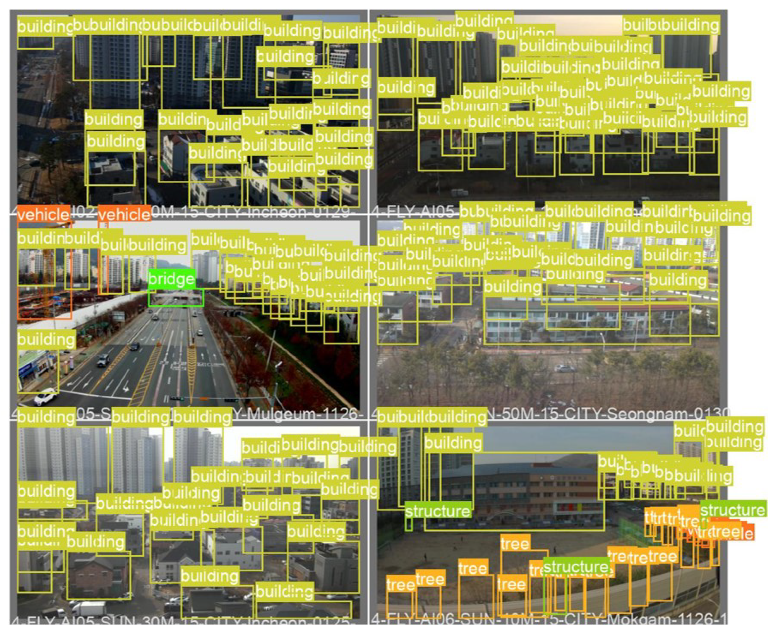
In Figure 5, we show that the recognized objects were mostly trees and buildings. As they were photographed from the perspective of drones, many objects were detected at once, and in particular, the recognition of objects as trees, apartment complexes, and general housing complexes accounted for the majority. The number of trees was the most at the horizon 0° angle of the drones, followed by buildings, streetlights, and traffic lights. In Figure 6, the coordinates of the objects were mostly positioned at the bottom 1/3 of the image and scattered with small sizes. In that case, it can be seen that the filtering was suitable because there were few objects to be detected when flying at a higheraltitude. In Figure 7, the confusion matrix can be checked after training the model by comparing the expected Y value produced by adding the X value into the model data with the actual Y value, in other words, as a result, showing how good the prediction was.
To evaluate the object detection models, the mean Average Precision (mAP)was used. The mAP is a score calculated by comparing the ground-truth bounding box to the detected box. The higher the score, the better the model’s detection accuracy is. Table 4 shows the model’s average accuracy of 0.7284 based on mAP_0.5 and 0.4846 based on mAP_0.5:0.95, and the best epoch showed an accuracy of 0.7968 based on mAP_0.5, having satisfactory performance. We used the latest version of YOLOv5s. The experimental results in this table are meant to show that using the YOLOv5s model on a UAV is possible and has a good object detection performance.
Figure 8 shows that the accuracy of each object was found to be high in the order of bridges (0.995), buildings (0.949), and vehicles (0.793). In particular, bridges and buildings are big, so they exhibited high accuracy even when resizing. As a result of the performance evaluation, the validation data for the verification of the 20 m, 40 m, and 60 m sections were detected.
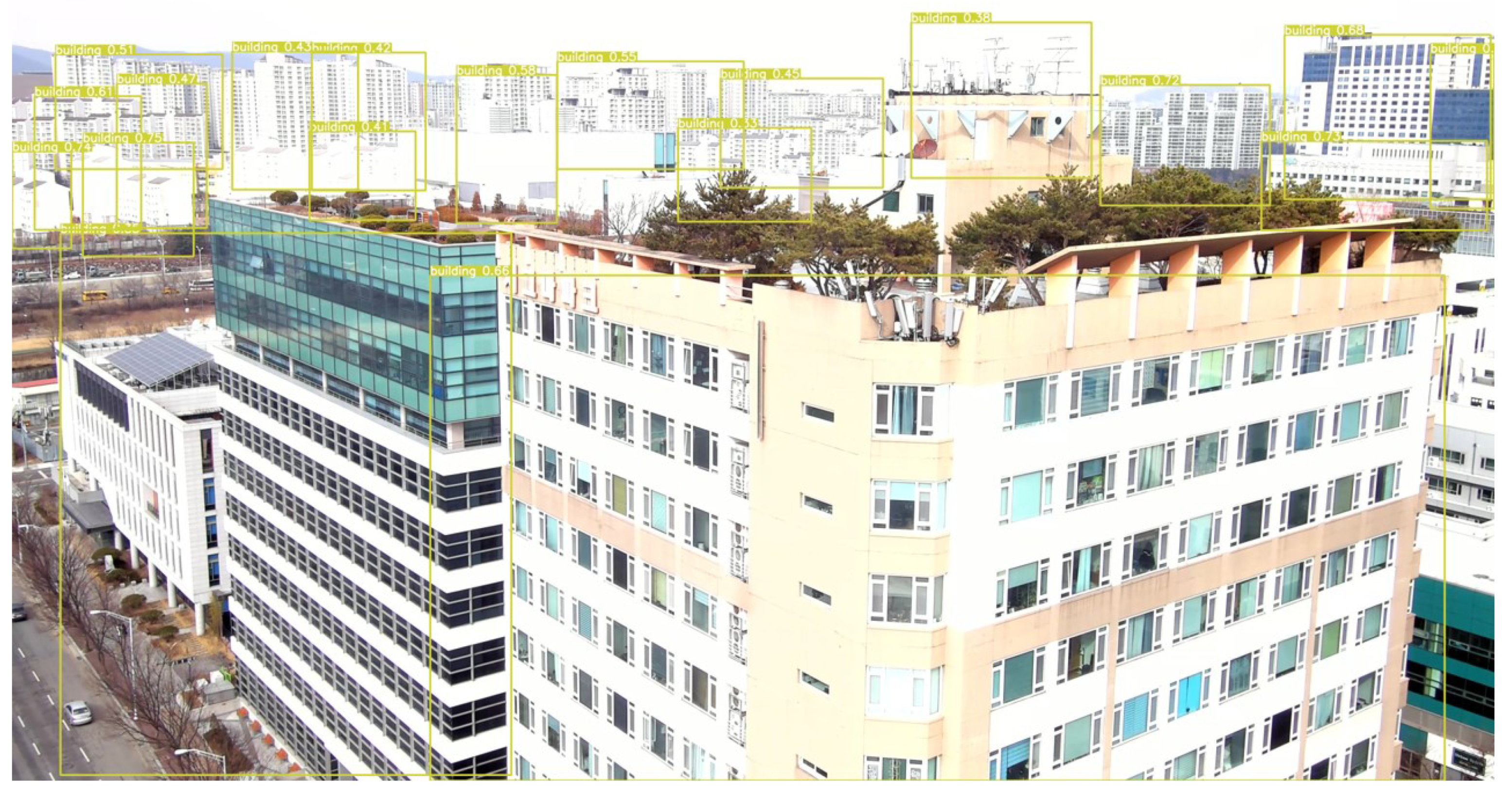
A feature of an altitude of 20 m is that various objects were detected. Objects such as people, vehicles, trees, buildings, and streetlights/traffic lights were all detected. In the case of a low altitude, there were small-sized objects, so resizing the input image reduced the accuracy, and filtering out small-sized items with filtering techniques did not work at this altitude. From an altitude of 40 m, large objects such as buildings and bridges were detected. This is the section where full-scale filtering began from this altitude and speed improvement occurred. The input image was 640 × 640 px, and the detection speed was 108.8 ms. We also reduced the detection time by resizing the image to 320 × 320 px in order to make it real-time. When filtering at a height of 20 m, 40 m, and 60 m, the result of employing 320 × 320 px was as presented in Figure 9. The reference process showed a 32.6% improvement from 108.8 ms to 81.4 ms. Therefore, it is important to avoid excessive resizing at low and medium altitudes and enter it at an optimized resolution. At an altitude of 60 m, the number of objects was reduced, and the majority of them were buildings. For the validation data, 120 photographed images wherein only building objects were detected at 60 m were extracted and evaluated randomly, and the results were compared before and after filtering using the same data. Among the results, there were 2835 objects detected before filtering, 23.6 objects per image, and after filtering, 2669 objects were detected, 22.2 objects per image. This shows an average error of 1.4. However, the object inference time before filtering was 0.105 s on average, and the object inference time after filtering was 0.066 s, showing a 59% performance improvement in the detection time.
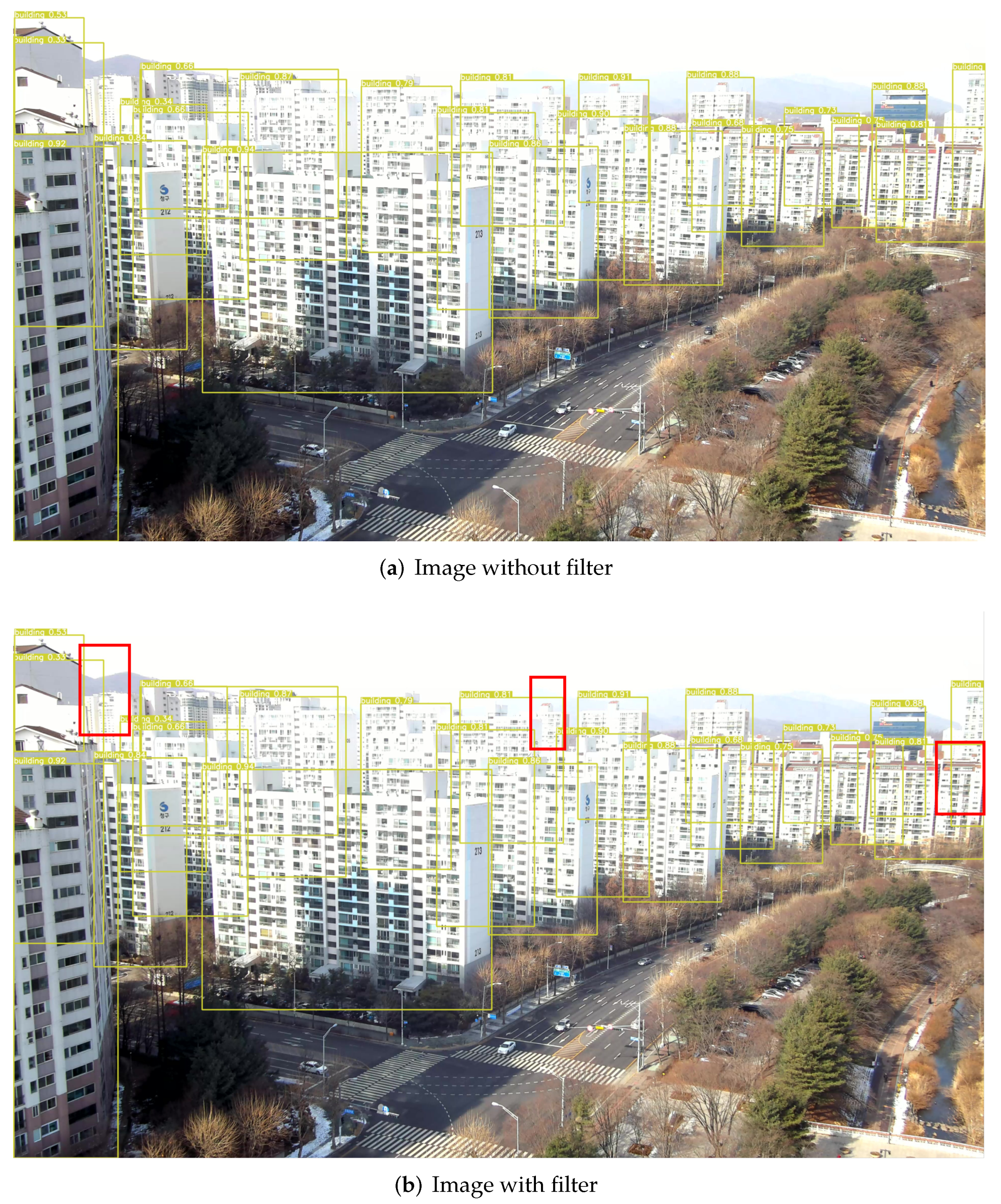
Figure 10 indicates the performance improvement after using filtering. To confirm whether this reduction in accuracy affected the flight, the detection location and shape of the object were analyzed. The red zone in Figure 10b shows the location and distribution of the reduced objects. As a result of the great accuracy with which the objects in the images in the front were identified, the identification rate of the distant objects in the images was reduced. In other words, when a drone flew, even if some objects over a long distance were not detected, the recognition speed of the front objects was high, so autonomous flight was possible without affecting the collision avoidance. In particular, it was possible to reduce the error rate by reducing the size from 640 × 640 px to 480 × 480 px.
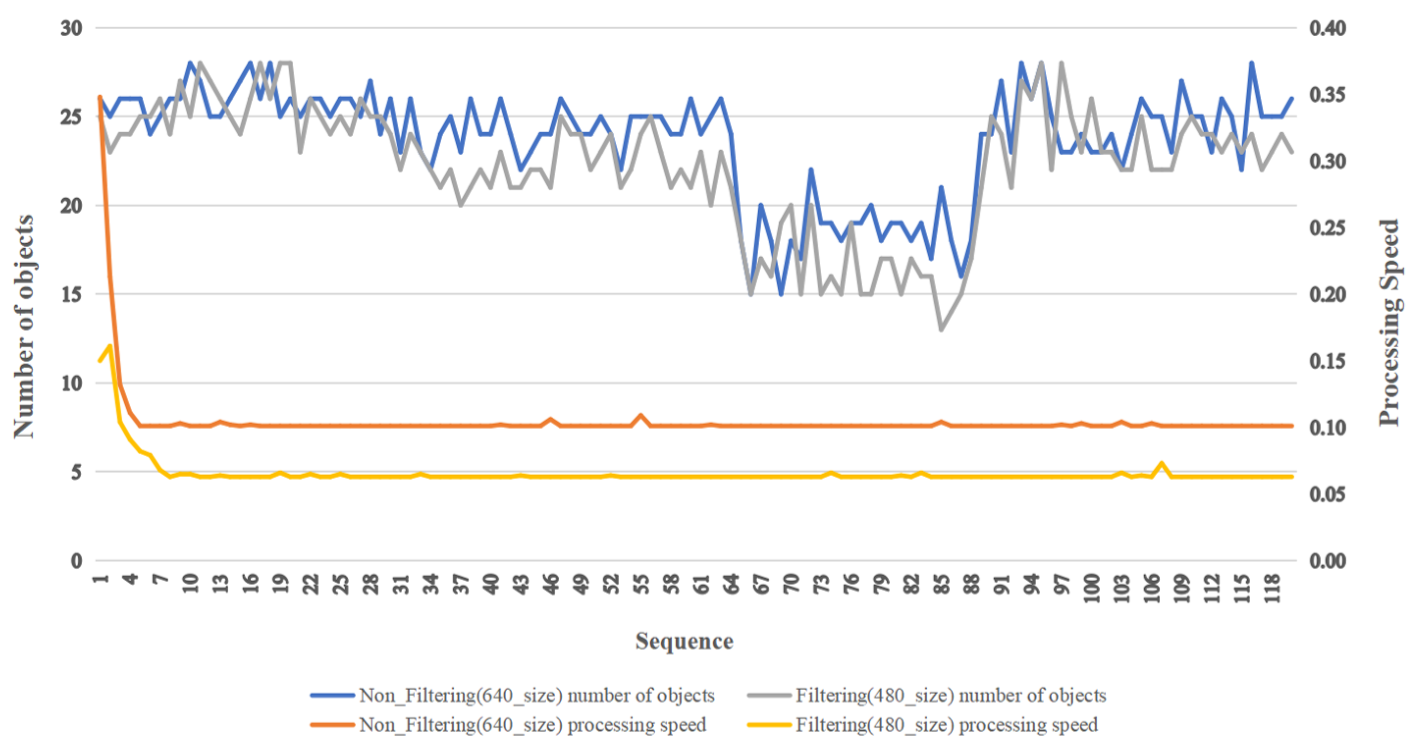
Table 5 and Figure 11 compare the filtering process and non-filtering process for each sequence. We used a filtering technique to filter objects such as people and vehicles when they were detected by the UAV at a high altitude; the size of these objects was very small in the images, but they were detected with no use of filteringwhen object detection was performed. The filtering technique was used because we wanted to remove small objects from the scene, which sped up the object detection. The reason we employed filters was to reduce the amount of effort spent detecting small-sized objects by deleting them. The initial sequence did not act as a large variable, as the data processing speed was partially delayed thereafter, but this would not act as a large variable as a result of the system environment irrespective of whether filtering was performed or not.
5. Conclusions
Our method aimed to increase the processing speed by reducing the number of pixels in the image while preserving the accuracy. The average inference time before filtering was 0.105 s at 60 m, and the inference time after filtering was decreased to 0.066 s, indicating a performance gain of roughly 59%. When the background was overlapping at a long distance, the accuracy may suffer, but it did not prevent the drones from recognizing objects in front of them, indicating that autonomous flight was possible. The results of the experiment may be seen at altitudes of 40 m and 60 m. Because of not only the overlap between the background and the object, but also the movement of people or vehicles, the accuracy at a low altitude was reduced more than the higher altitudes.
In the future, we will first acquire data from an altitude of 60 m to an actual height of 150 m, as determined under the law, and demonstrate this by including objects added there. Additional objects include mountains and hills and the transmission towers and transmission lines on top of them, and because the object size is large, it is expected to show high performance through filtering as in the current study. In the case of power transmission towers and power transmission lines, since magnetic fields are generated around them, a short-range flight can cause compass sensor errors. Therefore, it must be flown more than 20 m away. In the case of transmission lines, these are relatively thin objects, and their color is also close to black. In this case, depending on the environment, that is when the amount of light is low or when the object appears to overlap with a mountain in the background, the recognition rate may decrease, so many data should be obtained in consideration of various times of the dayand shooting angles. Second, drones are gradually evolving with the development of computers, and their value is increasing with the use of deep learning, while they are becoming more economical and more miniaturized. Future research aims to implement more accurate and faster autonomous flight by applying reinforcement learning in the filtering techniques and obtaining higher accuracy.
Author Contributions
Conceptualization, Y.L., J.A. and I.J.; methodology, Y.L.; software, Y.L.; validation, Y.L., J.A. and I.J.; investigation, Y.L. and J.A.; resources, Y.L., J.A.; data curation, Y.L.; writing—original draft preparation, Y.L. and J.A.; writing—review and editing, J.A. and I.J.; visualization, Y.L. and J.A.; supervision, I.J.; project administration, I.J.; funding acquisition, I.J. All authors have read and agreed to the published version of the manuscript.
Funding
This work was supported by the Institute of Information & Communications Technology Planning & Evaluation (IITP) grant funded by the Korea government (MSIT) (No. 2020-0-00107, Development of the technology to automate the recommendations for big data analytic models that define data characteristics and problems).
Institutional Review Board Statement
Not applicable.
Informed Consent Statement
Not applicable.
Data Availability Statement
Not applicable.
Conflicts of Interest
The authors declare no conflict of interest.
References
- Castle, R.O.; Klein, G.; Murray, D.W. Combining monoSLAM with object recognition for scene augmentation using a wearable camera. Image Vis. Comput. 2010, 28, 1548–1556. [Google Scholar] [CrossRef]
- Naikal, N.; Yang, A.Y.; Sastry, S.S. Towards an efficient distributed object recognition system in wireless smart camera networks. In Proceedings of the 2010 13th International Conference on Information Fusion, Edinburgh, UK, 26–29 July 2010; IEEE: Piscataway, NJ, USA, 2010; pp. 1–8. [Google Scholar]
- Yang, A.Y.; Maji, S.; Christoudias, C.M.; Darrell, T.; Malik, J.; Sastry, S.S. Multiple-view object recognition in band-limited distributed camera networks. In Proceedings of the 2009 Third ACM/IEEE International Conference on Distributed Smart Cameras (ICDSC), Como, Italy, 30 August–2 September 2009; IEEE: Piscataway, NJ, USA, 2009; pp. 1–8. [Google Scholar]
- Ren, Z.; Meng, J.; Yuan, J. Depth camera based hand gesture recognition and its applications in Human-Computer-Interaction. In Proceedings of the 2011 8th International Conference on Information, Communications Signal Processing, Singapore, 13–16 December 2011; pp. 1–5. [Google Scholar] [CrossRef]
- Xia, L.; Aggarwal, J. Spatio-temporal depth cuboid similarity feature for activity recognition using depth camera. In Proceedings of the IEEE Conference on Computer Vision and Pattern Recognition, Portland, OR, USA, 23–28 June 2013; pp. 2834–2841. [Google Scholar]
- Tham, J.S.; Chang, Y.C.; Fauzi, M.F.A.; Gwak, J. Object recognition using depth information of a consumer depth camera. In Proceedings of the 2015 International Conference on Control, Automation and Information Sciences (ICCAIS), Changshu, China, 29–31 October 2015; IEEE: Piscataway, NJ, USA, 2015; pp. 203–208. [Google Scholar]
- Melotti, G.; Premebida, C.; Gonçalves, N. Multimodal deep-learning for object recognition combining camera and LIDAR data. In Proceedings of the 2020 IEEE International Conference on Autonomous Robot Systems and Competitions (ICARSC), Ponta Delgada, Portugal, 15–17 April 2020; IEEE: Piscataway, NJ, USA, 2020; pp. 177–182. [Google Scholar]
- Matei, B.C.; Tan, Y.; Sawhney, H.S.; Kumar, R. Rapid and scalable 3D object recognition using LIDAR data. In Proceedings of the Automatic Target Recognition XVI; International Society for Optics and Photonics: Bellingham, DC, USA, 2006; Volume 6234, p. 623401. [Google Scholar]
- Watanabe, S.; Yoneyama, M. An ultrasonic visual sensor for three-dimensional object recognition using neural networks. IEEE Trans. Robot. Autom. 1992, 8, 240–249. [Google Scholar] [CrossRef]
- Huang, Q.; Yang, F.; Liu, L.; Li, X. Automatic segmentation of breast lesions for interaction in ultrasonic computer-aided diagnosis. Inf. Sci. 2015, 314, 293–310. [Google Scholar] [CrossRef]
- Heuer, H.; Breiter, A. More Than Accuracy: Towards Trustworthy Machine Learning Interfaces for Object Recognition. In Proceedings of the 28th ACM Conference on User Modeling, Adaptation and Personalization, Genoa, Italy, 12–18 July 2020; pp. 298–302. [Google Scholar]
- Mittal, P.; Sharma, A.; Singh, R. Deep learning-based object detection in low-altitude UAV datasets: A survey. Image Vis. Comput. 2020, 104, 104046. [Google Scholar] [CrossRef]
- Lu, X.; Kang, X.; Nishide, S.; Ren, F. Object detection based on SSD-ResNet. In Proceedings of the 2019 IEEE 6th International Conference on Cloud Computing and Intelligence Systems (CCIS), Singapore, 19–21 December 2019; IEEE: Piscataway, NJ, USA, 2019; pp. 89–92. [Google Scholar]
- Ali, H.; Khursheed, M.; Fatima, S.K.; Shuja, S.M.; Noor, S. Object recognition for dental instruments using SSD-MobileNet. In Proceedings of the 2019 International Conference on Information Science and Communication Technology (ICISCT), Karachi, Pakistan, 9–10 March 2019; IEEE: Piscataway, NJ, USA, 2019; pp. 1–6. [Google Scholar]
- Redmon, J.; Farhadi, A. Yolov3: An incremental improvement. arXiv 2018, arXiv:1804.02767. [Google Scholar]
- Fang, Y.; Guo, X.; Chen, K.; Zhou, Z.; Ye, Q. Accurate and Automated Detection of Surface Knots on Sawn Timbers Using YOLO-V5 Model. BioResources 2021, 16, 5390–5406. [Google Scholar] [CrossRef]
- Zhang, C.; Han, Z.; Fu, H.; Zhou, J.T.; Hu, Q. CPM-Nets: Cross Partial Multi-View Networks. August 2019. Available online: https://proceedings.neurips.cc/paper/2019/hash/11b9842e0a271ff252c1903e7132cd68-Abstract.html (accessed on 6 March 2022).
- Taketomi, T.; Uchiyama, H.; Ikeda, S. Visual SLAM algorithms: A survey from 2010 to 2016. IPSJ Trans. Comput. Vis. Appl. 2017, 9, 16. [Google Scholar] [CrossRef]
- Mur-Artal, R.; Tardós, J.D. Orb-slam2: An open-source slam system for monocular, stereo, and rgb-d cameras. IEEE Trans. Robot. 2017, 33, 1255–1262. [Google Scholar] [CrossRef] [Green Version]
- Xu, W.; Yan, C.; Jia, W.; Ji, X.; Liu, J. Analyzing and enhancing the security of ultrasonic sensors for autonomous vehicles. IEEE Internet Things J. 2018, 5, 5015–5029. [Google Scholar] [CrossRef]
- Ismail, R.; Omar, Z.; Suaibun, S. Obstacle-avoiding robot with IR and PIR motion sensors. In IOP Conference Series: Materials Science and Engineering; IOP Publishing: Bristol, UK, 2016; Volume 152, p. 012064. [Google Scholar]
- Walambe, R.; Marathe, A.; Kotecha, K. Multiscale object detection from drone imagery using ensemble transfer learning. Drones 2021, 5, 66. [Google Scholar] [CrossRef]
- Ye, X.; Chen, S.; Xu, R. DPNet: Detail-preserving network for high quality monocular depth estimation. Pattern Recognit. 2021, 109, 107578. [Google Scholar] [CrossRef]
- Wang, Y.; Solomon, J.M. Prnet: Self-supervised learning for partial-to-partial registration. arXiv 2019, arXiv:1910.12240. [Google Scholar]
- Joseph Nelson, J.S. YOLOv5 is Here: State-of-the-Art Object Detection at 140 FPS. Available online: https://blog.roboflow.com/yolov5-is-here/ (accessed on 10 June 2020).
Figure 1.
An example of the frames per second. The frames of detection per second is referred to as FPS, and if detection is processed at 30 frames per second, this is referred to as 30 FPS.
Figure 1.
An example of the frames per second. The frames of detection per second is referred to as FPS, and if detection is processed at 30 frames per second, this is referred to as 30 FPS.

Figure 2.
The comparison of various deep learning inference networks’ performance, using FP16 precision and a batch size of 1.
Figure 2.
The comparison of various deep learning inference networks’ performance, using FP16 precision and a batch size of 1.

Figure 3.
The process of creating an avoidance route for VAF. When the drone takes off, the drone receives data in real-time, then transmits the data to the flight controller. Following that, we use our filtering method to remove the small-sized objects, which may cause the the detecting time to become slower, then detect the object and create an avoidance route.

Figure 4.
Performance comparison between YOLOv5 and EfficientDet [25]. COCO AP Val denotes the mAP metric measured on the COCO val2017 dataset over various inference sizes from 256 to 1536. The GPU speed measures the average inference time per image on the COCO val2017 dataset. It shows that the YOLOv5 family is much faster than EfficientDet with a good performance.

Figure 5.
The result of object detection on VAF. The objects detected by VAF mainly consist of trees and buildings.
Figure 5.
The result of object detection on VAF. The objects detected by VAF mainly consist of trees and buildings.

Figure 6.
The result of objects’ distribution. The coordinates of the object are largely near the bottom of the image and are distributed over a small region, indicating that when flying at a high altitude, only a few objects need to be recognized.
Figure 6.
The result of objects’ distribution. The coordinates of the object are largely near the bottom of the image and are distributed over a small region, indicating that when flying at a high altitude, only a few objects need to be recognized.

Figure 7.
The confusion matrix after training the model. Vehicles, bridges, and buildings were able to be accurately detected, demonstrating how good the prediction was.
Figure 7.
The confusion matrix after training the model. Vehicles, bridges, and buildings were able to be accurately detected, demonstrating how good the prediction was.

Figure 8.
The result of using the YOLOv5s model. The YOLOv5 model performs well. Bridges and buildings, in particular, are massive structures that require tremendous precision even when scaling.
Figure 8.
The result of using the YOLOv5s model. The YOLOv5 model performs well. Bridges and buildings, in particular, are massive structures that require tremendous precision even when scaling.

Figure 9.
The results of the 20 M, 40 M, and 60 M detections. A variety of objects are detected, such as people, vehicles, trees, and buildings. However, when creating avoidance routes, small objects do not need to be detected, making the model slower at detection.
Figure 9.
The results of the 20 M, 40 M, and 60 M detections. A variety of objects are detected, such as people, vehicles, trees, and buildings. However, when creating avoidance routes, small objects do not need to be detected, making the model slower at detection.


Figure 10.
(a) Image without the filter. The buildings in the distance are also detected in this image. (b) Image with the filter. We used the filter to filter out the distant buildings. This is because the distant buildings do not need to be detected when creating the avoidance route.
Figure 10.
(a) Image without the filter. The buildings in the distance are also detected in this image. (b) Image with the filter. We used the filter to filter out the distant buildings. This is because the distant buildings do not need to be detected when creating the avoidance route.

Figure 11.
Comparison results before and after filtering. The experimental results show a significant increase in the speed of object detection. We can quickly boost the speed of detection and create avoidance routes in real-time by employing our method.
Figure 11.
Comparison results before and after filtering. The experimental results show a significant increase in the speed of object detection. We can quickly boost the speed of detection and create avoidance routes in real-time by employing our method.


Table 1.
Workstation configuration for the experiment.
| Software or Hardware | Specification |
|---|---|
| OS | Linux Ubuntu 20.04 |
| CPU | Intel Core [email protected] Hz |
| GPU | GeForce RTX 1080 Ti *4EA |
| RAM | DDR4 48 GB |
Table 2.
Frame speed comparison of the deep learning models.
| Model | mAP | FLOPS | FPS |
|---|---|---|---|
| SSD300 | 41.2 | - | 46 |
| SSD321 | 45.4 | - | 16 |
| SSD500 | 46.5 | - | 19 |
| SSD513 | 50.4 | - | 8 |
| DSSD321 | 46.1 | - | 12 |
| Tiny YOLO | 23.7 | 5.41 Bn | 244 |
| YOLOv2 608x608 | 48.1 | 62.94 Bn | 40 |
| YOLOv3-320 | 51.5 | 38.97 Bn | 45 |
| YOLOv3-416 | 55.3 | 65.86 Bn | 35 |
| YOLOv3-608 | 57.9 | 140.69 Bn | 20 |
| YOLOv3-tiny | 33.1 | 5.56 Bn | 220 |
| YOLOv3-spp | 60.6 | 141.45 Bn | 20 |
| R-FCN | 51.9 | - | 12 |
| FPN FRCN | 59.1 | - | 6 |
| RetinaNet-50-500 | 50.9 | - | 14 |
| RetinaNet-101-500 | 53.1 | - | 11 |
| RetinaNet-101-800 | 57.5 | - | 5 |
Table 3.
The parameters of the training model.
| Model | Batch Size | Epochs |
|---|---|---|
| YOLOv5s | 64 | 300 |
Table 4.
The result of training the YOLOv5s model.
| Train | Validation | ||||
|---|---|---|---|---|---|
| Box_loss | Cls_loss | Obj_loss | Box_loss | Cls_loss | Obj_loss |
| 0.0448 | 0.0037 | 0.2296 | 0.0378 | 0.0021 | 0.2191 |
| Metric | |||||
| mAP_0.5 | Map_0.5:0.95 | Precision | Recall | ||
| 0.7284 | 0.4846 | 0.5739 | 0.8617 | ||
Table 5.
Performance comparison table before and after filtering.
| Sequence | Non_Filtering (640 × 640 px) | Filtering (480 × 480 px) | Object Error | ||
|---|---|---|---|---|---|
| Number of Objects | Processing Speed | Number of Objects | Processing Speed | ||
| 1 | 26 | 0.348 ms | 25 | 0.150 ms | 1 |
| 2 | 25 | 0.213 ms | 23 | 0.161 ms | 2 |
| 3 | 26 | 0.132 ms | 24 | 0.104 ms | 2 |
| 4 | 26 | 0.111 ms | 24 | 0.091 ms | 2 |
| 5 | 26 | 0.101 ms | 25 | 0.082 ms | 1 |
| 6 | 24 | 0.101 ms | 25 | 0.079 ms | 1 |
| 7 | 25 | 0.101 ms | 26 | 0.068 ms | 1 |
| 8 | 26 | 0.101 ms | 24 | 0.063 ms | 2 |
| 9 | 26 | 0.103 ms | 27 | 0.065 ms | 1 |
| 10 | 28 | 0.101 ms | 25 | 0.065 ms | 3 |
| 11 | 27 | 0.101 ms | 28 | 0.063 ms | 1 |
| 12 | 25 | 0.101 ms | 27 | 0.063 ms | 2 |
| 13 | 25 | 0.104 ms | 26 | 0.064 ms | 1 |
| 14 | 26 | 0.102 ms | 25 | 0.063 ms | 1 |
| 15 | 27 | 0.101 ms | 24 | 0.063 ms | 3 |
| 16 | 28 | 0.102 ms | 26 | 0.063 ms | 2 |
| 17 | 26 | 0.101 ms | 28 | 0.063 ms | 2 |
| 18 | 28 | 0.101 ms | 26 | 0.063 ms | 2 |
| 19 | 25 | 0.101 ms | 28 | 0.066 ms | 3 |
| 20 | 26 | 0.101 ms | 28 | 0.063 ms | 2 |
| 21 | 25 | 0.101 ms | 23 | 0.063 ms | 2 |
| 22 | 26 | 0.101 ms | 26 | 0.065 ms | 0 |
| 23 | 26 | 0.101 ms | 25 | 0.063 ms | 1 |
| 24 | 25 | 0.101 ms | 24 | 0.063 ms | 1 |
| 25 | 26 | 0.101 ms | 25 | 0.065 ms | 1 |
| 26 | 26 | 0.101 ms | 24 | 0.063 ms | 2 |
| 27 | 25 | 0.101 ms | 26 | 0.063 ms | 1 |
| 28 | 27 | 0.101 ms | 25 | 0.063 ms | 2 |
| 29 | 24 | 0.101 ms | 25 | 0.063 ms | 1 |
| 30 | 26 | 0.101 ms | 24 | 0.063 ms | 2 |
Publisher’s Note: MDPI stays neutral with regard to jurisdictional claims in published maps and institutional affiliations. |
© 2022 by the authors. Licensee MDPI, Basel, Switzerland. This article is an open access article distributed under the terms and conditions of the Creative Commons Attribution (CC BY) license (https://creativecommons.org/licenses/by/4.0/).
Share and Cite
MDPI and ACS Style
Lee, Y.; An, J.; Joe, I. Deep-Learning-Based Object Filtering According to Altitude for Improvement of Obstacle Recognition during Autonomous Flight. Remote Sens. 2022, 14, 1378. https://doi.org/10.3390/rs14061378
AMA Style
Lee Y, An J, Joe I. Deep-Learning-Based Object Filtering According to Altitude for Improvement of Obstacle Recognition during Autonomous Flight. Remote Sensing. 2022; 14(6):1378. https://doi.org/10.3390/rs14061378
Chicago/Turabian StyleLee, Yongwoo, Junkang An, and Inwhee Joe. 2022. "Deep-Learning-Based Object Filtering According to Altitude for Improvement of Obstacle Recognition during Autonomous Flight" Remote Sensing 14, no. 6: 1378. https://doi.org/10.3390/rs14061378
Note that from the first issue of 2016, this journal uses article numbers instead of page numbers. See further details here.